We present the main ideas behind Variational Inference. In particular, we examine applications such as Variational Autoencoders, Expectation–Maximization and Diffusion Models.
- Energy Formulation and Mixtures
- Variational Inequalities
- Applications
- Variational Autoencoder
- Vanilla Diffusion
- Model
- Tractability
- Forward Recurrence Relations
- Cummulative Shrink and Noise Factors
- General Covariance Calculation
- Backward Inference
- Incremental Denoiser
- Dependency on the initial condition
- Initial Condition Sensitivity
- Direct Denoiser
- Noise Predictor
- What is needed in the end?
- Further Simplifications
The general idea is that we have data points \(x_i\) in a set \(X\) for which we try and fit a probability distribution \(p(x)\). This means that we try and maximize \[ \max_{P \in \mathcal{P}} \sum_i \log(p(x_i)) \] where \(\mathcal{P}\) is a statistical manifold of probability distributions over the set \(X\), which purpose is to regularise, so as to avoid overfitting.
One way to achieve this is to decompose \(p\) in a mixture, that is \[ p(x) = \int p(x|z) p(z) \dd z \] The variable \(z\) is a latent variable, the probability \(p(z)\) is a prior, and the distributions \(p(x|z)\) for every \(z\) can be interpreted as decoders. In this context, the probability \(p(z|x)\) is an “optimal encoder”.
Energy Formulation and Mixtures
Assume first that
\[ \log(p(x,z)) = E(x,z) - \bar{E} \]
where \(\bar{E}\) is a normalisation scalar defined by \[ \bar{E} := \log\left(\int \exp\left(E(x,z)\right) \dd x \dd z\right) \]
Where does the Energy come from?
You can always define the energy as \(E(x,z) = \log(p(x,z))\), under the minor assumption that the probability is non-zero (it is a minor assumption, because we can always add a measure on that support in all the integrals). Here we allow the energy \(E\) to be proportional to the log-probability. It is very convenient because we don’t need to think about the normalisation constant which is defined by \(\bar{E}\).
Then one can check that
\begin{align} \log(p(x)) &= \log\left(\int p(x,z) \dd z\right) \\ &= \log\left(\int \exp\left(E(x,z) - \bar{E}\right) \dd z\right) \\ &= \bar{E}(x) - \bar{E} \end{align}
where
\[ \bar{E}(x) := \log\left(\int \exp\left(E(x,z) \dd z\right)\right) \]
And finally, for a fixed \(x\),
\begin{align} \log (p(z|x)) &= \log(p(x,z)) - \log(p(x)) \\ &= E(x,z) - \bar{E} -(\bar{E}(x) - \bar{E}) \\ &= E(x,z) - \bar{E}(x) \end{align}
So we finally obtained that:
\[ \log(p(x)) = \bar{E}(x) - \bar{E} \]
and
\[ \log(p(z|x)) = E(x,z) - \bar{E}(x) \]
Thermodynamical Interpretation
If \(x\) denotes the external parameters, such as the volume, for instance, whereas \(z\) denotes internal parameters. The identity above shows that the free energy at a fixed external variable value \(x\) is exactly the quantity \(\bar{E}(x)\).
Variational Inequalities
The “inequalities” below are in fact equalities of the form \[ A = \underbrace{D(\cdots)}_{\geq 0} + B \] where \(D(\cdots)\) denotes a divergence, which implies, but is more accurate than, \[ A \geq B . \]
Free Energy
Now, the main “variational free energy” inequality comes by expanding the divergence between an arbitrary distribution \(q(z)\) over \(z\) (that we will call the “approximate encoder” for \(x\)) and the posterior distribution \(p(z|x)\): \begin{align} D(q(z) || p(z|x)) &= -H(q) - \langle q(z), \log(p(z|x)) \rangle \\ &= -H(q) +\bar{E}(x) - \langle q(z), E(x,z) \rangle \end{align} which can be rewritten as
\[ \bar{E}(x) = \underbrace{D(q(z) || p(z|x))}_{\geq 0} + \langle q(z), E(x,z) \rangle + H(q) \]
We can choose the approximate encoder \(q\) to be the optimal encoder \(p(z|x)\), so, \(q(z) = p(z|x)\), in this equation and obtain simply
\[ \bar{E}(x) = \langle p(z|x), E(x,z) \rangle + H(p(z|x)) \]
Thermodynamical Interpretation
This is the familiar equation in thermodynamics, typically denoted \(A = U - TS\), relating
- the entropy \(H(p(z|x))\)
- the mean energy \(\langle p(z|x), E(x,z) \rangle\)
- the free energy \(\bar{E}(x)\)
for a fixed external parameter (here, the fixed value \(x\)).
Variational Free Energy
By analogy, we can define the quantity \[ \bar{E}_q(x) := \langle q(z), E(x,z) \rangle + H(q) \] and call it the “variational free energy” associated to the distribution \(q(z)\). We then have \[ \bar{E}(x) = \underbrace{D(q(z) || p(z|x))}_{\geq 0} + \bar{E}_q(x) \] or simply: \[ \bar{E}(x) \geq \bar{E}_q(x) \] for all distributions \(q\) (approximate encoders) over the latent space.
Thermodynamical Interpretation
In thermodynamics, this variational free energy \(\bar{E}_q\) is the free energy of a system (described by the probability distribution \(q\)) which is not at equilibrium. At equilibrium, the system should fulfil \(q = p(z|x)\). (Remember that in all those calculations, the data point \(x\), or external variable \(x\), is fixed)
Expectation-Maximisation Equality
By substracting the scalar \(\bar{E}\) in the last formulation, we obtain
\begin{align} \log(p(x)) &= D(q(z) || p(z|x)) \\ &+ \underbrace{\langle q(z), \log(p(x,z)) \rangle + H(q)}_{\bar{E}_q(x) - \bar{E}} \end{align}
The idea behind the expectation-maximization algorithm is essentially as follows:
- Maximisation step Fix the decoder \(p\), so \(\log(p(x))\) is fixed, and then maximise \(\bar{E}_q(x)\) by varying the approximate encoder \(q\), which amounts to maximise \(\bar{E}_q - \bar{E}\). The maximum is achieved when the approximate encoder is the optimal encoder, that is, \(q(z) = p(z|x)\).
- Expectation step Fix then the approximate encoder \(q\) and maximise \(\bar{E}_q(x)-\bar{E}\) by changing the decoder \(p(x,z)\). Since the approximate encoder \(q\) is now fixed, this amounts to maximising \(\langle q(z), \log(p(x,z)) \rangle\) by varying \(p(x,z)\) on the manifold \(\mathcal{P}\).
Example: Fuzzy Clustering
Fuzzy clustering (or “soft K-means”) is an application of that idea.
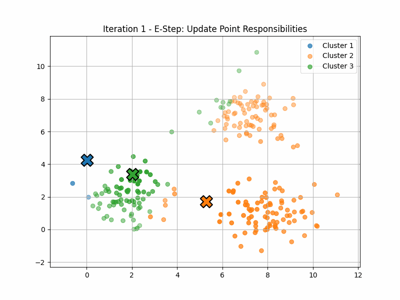
Here, the manifold \(\mathcal{P}\) has six dimensions, corresponding to the locations of the three centroids.
The maximisation step computes \(p(z|x)\) for each of the data points. This quantity is often called the responsability of the latent variable \(z\) for that data point \(x\).
The expectation step now finds the point on \(\mathcal{P}\) that maximises \(\langle q(z), \log(p(x,z)) \rangle\).
Autoencoder Inequality
The other (equivalent) variational inequality is:
\begin{align} \log(p(x)) &= \underbrace{D(q(z) || p(z|x))}_{\geq 0}\\ &+ \langle q(z), \log(p(x|z)) \rangle - D(q(z) || p(z)) \end{align}
This is because, by expanding the last divergence and using the identities above, the last variational equality amounts to
\begin{align}
\bar{E}(x) - \bar{E}
=
& D(q(z) || p(z|x)) \\
&+
\langle q(z), \underbrace{E(x,z)-\bar{E}(z)}_{\log(p(x|z))} \rangle
\
+ H(q)
\\
&+ \langle q(z), \underbrace{\bar{E}(z) - \bar{E}}_{\log(p(z))} \rangle
\end{align}
Again, if we use the optimal encoder \(q(z) = p(z|x)\) we obtain an interesting equality, namely
\[ \log(p(x)) = \langle p(z|x), \log(p(x|z)) \rangle - D(p(z|x) || p(z)) \]
This can be roughly interpreted as follows. If the prior \(p(z)\) is fixed, then the maximum likelihood must use as much weight as possible in the posterior distribution \(p(z|x)\).
The strategy of the variational autoencoder is to fix a prior distribution \(p(z)\) in a statistical manifold where the divergence between two points can be computed explicitly. One then restrict the approximate encoder \(q(z)\) to belong to that statistical manifold.
Diffusion Models
In this case, we make the assumption that the latent variable \(z\) splits into \(z_1,\ldots, z_T\). We assume that both the approximate encoder \(q\) and the fitting probability \(p\) have the Markov chain property, so \[ q(z_1, \ldots,z_T) = q(z_1|z_2)\cdots q(z_{T-1}|z_T)q(z_T) \] \[ p(x,z_1, \ldots,z_T) = p(x|z_1)p(z_1|z_2)\cdots p(z_{T-1}|z_T)p(z_T) \] We then compute \[ p(x|z) = p(x|z_1) \] and \begin{align} (q(z)||p(z)) &= \Big\langle q(z), \sum_{k=1}^{T-1} D\left(q(z_{k}|z_{k+1})|| p(z_k|z_{k+1})\right) \\ & + D\left(q(z_T)||p(z_T)\right) \Big\rangle \end{align}
In the end, we get
\begin{align} \log(p(x)) &= D(q(z)|| p(z|x)) \\ & +\Big\langle q(z), \log\left(p(x|z_1)\right) \\ & - \sum_{k=1}^{T-1} D\left(q(z_{k}|z_{k+1})|| p(z_k|z_{k+1})\right) \Big\rangle \\ & - D\left(q(z_T)||p(z_T)\right) \end{align}
The idea is now that the approximate encoder \(q(z)\) is fixed (but depends on the data point \(x\)).
Applications
Variational Autoencoder
Model
The family of decoders \(\mathcal{P}\) is defined by specifying the prior \(p(z)\) and the conditional distributions \(p(x|z)\). In this case, the prior \(p(z)\) is fixed to an isotropic normal distribution in a latent space: \(p(z) \sim \mathcal{N}(\mu= 0, \sigma=\mathbf{1})\). The real decoder \(p(x|z)\) is typically normally distributed \(p(x|z) \sim \mathcal{N}(\mu_p(z), \sigma \mathbf{1})\) with a fixed real parameter \(\sigma\).
Now the family \(\mathcal{Q}\) is defined as follows. The approximate encoder \(q(z)\) depends on \(x\) and is also normally distributed \(q_x(z) \sim \mathcal{N}(\mu=\mu_q(x); \sigma=\Sigma_q(x))\). The variance \(\Sigma_q(x)\) is typically isotropic, so \(\Sigma_q(x) = \sigma_q(x) \mathbf{1}\), but with a trainable scaling parameter \(\sigma_q(x)\).
All the functions \(\mu_p(z)\), \(\mu_q(x)\) and \(\Sigma_q(x)\) are parameterized by neural networks.
Training is performed by picking a data point \(x\) (or a batch), and constructing the loss function: \[ L_x(p,q) := \langle q_x(z), -\log(p(x|z)) \rangle + D(q_x(z) || p(z)) \]
Tractability
Pathwise Gradient Estimation
The gradient (with respect to \(q\)) of the term \(\langle q(z), \log(p(x|z)) \rangle\) is, however, problematic to compute. The solution is to further assume that the latent statistical manifold can be obtained as the image of a family of random variables. So we assume that there is some distribution \(q_0\), and that any distribution \(q\) in the latent manifold \(\mathcal{Q}\) can be expressed as a push forward by a family of functions \(\Phi\) of a single reference distribution \(q_0\): \[ q = \Phi_* q_0 \] The term above becomes
\begin{align} \langle (\Phi_{\star} q_0)(z), \log(p(x|z)) \rangle &= \langle q_0(z), \Phi^{\star} \log(p(x|z)) \rangle \\ &=\langle q_0(z), \log(p(x|\Phi(z))) \rangle \end{align}
Explicit Divergences
One can compute the divergence between two normal distributions, one with covariance \(\Sigma_0\) and mean \(\mu_0\) and one with precision \(\Lambda_1\) and mean \(\mu_1\).
\[ D(p(x_0)|| p(x_1)) = D(\Sigma_0||\Lambda_1) + \frac{1}{2} |\mu_1 - \mu_0|^2_{\Lambda_1} \]
where \(D(\Sigma_0||\Lambda_1)\) is the divergence between two centered normal distributions of covariance \(\Sigma_0\) and precision \(\Lambda_1\). In dimension \(d\), that divergence is equal to
\[ D(\Sigma_0||\Lambda_1) = \frac{1}{2}\left(\mathrm{Tr}(\Lambda_1\Sigma_0) - d - \log(|\Lambda_1| |\Sigma_0|)\right) \]
and where we defined the norm
\[ |x|_{\Lambda}^2 := \langle \Lambda x, x \rangle \]
Vanilla Diffusion
Model
More precisely, assume that \(q_x(z_{k+1}|z_k)\) takes the form \[ q_x(z_{k+1}|z_k) \sim \mathcal{N}(\mu=\sqrt{\alpha_{k+1}}z_k; \sigma=\beta_{k+1}) \] for some parameters \(\beta_k \in (0,1)\) and \(\alpha_{k}\). As we shall see, one usually assumes \(\alpha_{k} = {1-\beta_{k}}\).
Further assume that \[q_x(z_1) \sim \mathcal{N}(\mu= x; \sigma= \beta_0) . \] We see that this approximate encoder is fixed, that is, not trainable, for a given point \(x\). Further, notice that \(q_x(z_{k+1}|z_k)\) does not depend on \(x\) at all, as it is just noise added to \(z_k\). The whole approximate encoder \(q_x\) depends on \(x\) only through \(q_x(z_1)\).
The true decoder \(p\) is modeled as \[ p(z_{k}|z_{k+1}) \sim \mathcal{N}(\mu=\mu_k(z_{k+1}); \sigma=\Sigma_k(z_{k+1})) \] as well as \[ p(x|z_1) \sim \mathcal{N}(\mu=\mu_0(z_1); \sigma=\Sigma_0(z_1)) \] and \[ p(z_T) \sim \mathcal{N}(\mu= 0; \sigma=\mathbf{1}) \] where \(\mu_k\) is a learned parameter and \(\Sigma_k\) is computed analytically.
Tractability
⚠️ Calculations Ahead ⚠️
To be clear, the aim of this section is to show that even if the incremental shrinking and noise coefficient are arbitrary, that is, not necessarily scalar, one can carry on all the necessary computations to evaluate the error term used for training. In practice, not only does one use scalar coefficients only, but one also ignores the scaling term thus computed in the end alltogether.
The bottom line is: read these calculations for your own enjoyment, but they are not very useful in practice.
Note that the model prescribes the distribution \(q\) as an encoder, although in the loss function we need it as a decoder. In other words, we need expressions for \(q(z_k|z_{k+1})\). This is, however, a rather simple task, since one can think of the sequence of random variables \(Z_k\), distributed according to the distribution \(q\), as being a linear combination of the previous one.
We assume that \[ Z_1 = x + \mathsf{B}_{1} \varepsilon_0 \] and \[ Z_{k+1} = \mathsf{A}_{k+1}Z_k + \mathsf{B}_{k+1}\varepsilon_{k} \]
We can think of \(\mathsf{A}_{k}\) as a incremental shrinking coefficient at time \(k\) and of \(\mathsf{B}_{k}\) as a incremental noise level, or time step at time \(k\).
Forward Recurrence Relations
First, moving forward, we obtain the following recurrence relations: \[ \mu[Z_{k+1}] = \mathsf{A}_{k+1}\mu[Z_k] \] and \[ \Sigma[Z_{k+1}] = \mathsf{A}_{k+1}\Sigma[Z_k]\mathsf{A}_{k+1}^{\ast} + \mathsf{B}_{k+1}\mathsf{B}_{k+1}^{\ast} \] with initial conditions \[ \mu[Z_0] = x \] and \[ \Sigma[Z_0] = 0 \]
Cummulative Shrink and Noise Factors
We see that the noisy variables \(Z_k\) can be expressed in terms of \(x\) and some standard normally distributed variable \(\varepsilon\) as \[ Z_k = \bar{\mathsf{A}}_{k} x + \bar{\mathsf{B}}_{k} \varepsilon \] and both \(\bar{\mathsf{A}}_{k}\) and \(\bar{\mathsf{B}}_{k}\) can be computed from the recursion above, by the equations \[\bar{\mathsf{A}}_{k} = \mathsf{A}_{k} \cdots \mathsf{A}_{1}\] and \[\bar{\mathsf{B}}_{k}\bar{\mathsf{B}}_{k}^{\ast} = \Sigma[Z_k] .\] We can think of \(\bar{\mathsf{A}}_{k}\) as the cummulative shrinking coefficient at time \(k\) and \(\bar{\mathsf{B}}_{k}\) as the cummulative noise level at time \(k\).
General Covariance Calculation
We compute the sequence \(I_k\) using the recurrence relation \[ I_{k+1} = \mathsf{A}_{k+1}I_{k}\mathsf{A}_{k+1}^{\ast} + \mathsf{B}_{k+1}\mathsf{B}_{k+1}^{\ast} \] with initial condition \(I_0\).
The forward recurrence relation for the covariance becomes \[ \Sigma[Z_{k+1}] - I_{k+1} = \mathsf{A}_{k+1}(\Sigma[Z_k] - I_k)\mathsf{A}_{k+1}^{\ast} \] and this gives in the end, using \(\Sigma[Z_0] = 0\) and the definition of \(\bar{\mathsf{A}}_{k}\): \[ \Sigma[Z_k] = I_k -\bar{\mathsf{A}}_{k}I_0 \bar{\mathsf{A}}_{k}^{\ast} \] So on top of the recurrence \[ \mathsf{B}_{k+1}\mathsf{B}_{k+1}^{\ast} = I_{k+1} - \mathsf{A}_{k+1}I_{k}\mathsf{A}_{k+1}^{\ast} \] we also have the equation \[ \bar{\mathsf{B}}_{k} \bar{\mathsf{B}}_{k}^{\ast} = I_k - \bar{\mathsf{A}}_{k}I_0\bar{\mathsf{A}}_{k}^{\ast} \]
Backward Inference
Now we need to move backward, and for this is it easier to use precision \(\Lambda\) (the inverse of the covariance) and the frequency \(f\) (product of precision and mean). Note first that we have, by definition \[ \Lambda[Z_k] = \Sigma[Z_k]^{-1} \] and \[ f[Z_k] = \Lambda[Z_k] \mu[Z_k] \]
Now for the conditional versions: \[ \Lambda[Z_k|z_{k+1}] = \Lambda[Z_k] + \mathsf{A}_{k+1}^{\ast}(\mathsf{B}_{k+1}\mathsf{B}_{k+1}^{\ast})^{-1} \mathsf{A}_{k+1} \] Note that the last quantity is constant, that is, independent of \(z_{k+1}\), so there is no need to train.
We compute finally \[ f[Z_k|z_{k+1}] = f[Z_k] + \mathsf{A}_{k+1}^{\ast}(\mathsf{B}_{k+1}\mathsf{B}_{k+1}^{\ast})^{-1} z_{k+1} \]
This allows to compute \(\mu[Z_k|z_{k+1}]\).
Incremental Denoiser
We assume that \(p(z_k|z_{k+1})\) has a fixed covariance \(\Sigma_k\) (or precision \(\Lambda_k\)). The divergence reduces to \[ D\Big(q(z_{k}|z_{k+1})|| p(z_k|z_{k+1})\Big) = \frac{1}{2}\big\|\mu_k - \mu[Z_k|z_{k+1}]\big\|^2_{\Lambda_k} + D(\Sigma[Z_k|z_{k+1}] || \Lambda_k) \] and the second term is a constant. We will now focus on the first term that is \[ L = \frac{1}{2}\big\|\mu_k - \mu[Z_k|z_{k+1}]\big\|^2_{\Lambda_k} \]
Dependency on the initial condition
Another idea is that the network directly predicts \(x\). Indeed, note that \(\mu[Z_k|z_{k+1}]\) is a linear combination of \(x\) and \(z_{k+1}\): \[ \mu[Z_k|z_{k+1}] = M_k x + N_k z_{k+1} \] with some known, fixed matrices \(M_k\) and \(N_k\). We call \(M_k\) the initial condition sensitivity. We will need a formula for \(M_k\), so let us compute it.
Initial Condition Sensitivity
We have: \[ \mu[Z_k] = \bar{\mathsf{A}}_{k} x \] And also \begin{align} f[Z_k|z_{k+1}] &= \Lambda[Z_k]\bar{\mathsf{A}}_{k} \\ &+ \mathsf{A}_{k+1}^{\ast}(\mathsf{B}_{k+1}\mathsf{B}_{k+1}^{\ast})^{-1} z_{k+1} \end{align} from which we deduce \[ M_k = \Sigma[Z_k|z_{k+1}] \Lambda[Z_k]\bar{\mathsf{A}}_{k} \]
Direct Denoiser
Suppose now that the network outputs a completely denoised point \(y(k, z_{k+1})\) such that \(\mu_k = M_k y(k, z_{k+1}) + N_k z_{k+1}\). We compute \( \mu_k - \mu[Z_k|z_{k+1}] = M_k (y(k, z_{k+1})-x)\) and if we define the constant, pulled-back precision \[\bar{\Lambda}_k := M_k^{\ast}\Lambda_k M_k \] the loss term \(L\) now becomes \[ L = \frac{1}{2} \|{ y(k,z_{k+1})-x }\|^2_{\bar{\Lambda}_k} \]
Noise Predictor
Note that, in the expression above, one takes the mean over \(z_{k+1}\), in other words, one has to regard \(z_{k+1}\) as a random variable. As we saw before, \(Z_{k+1} = \bar{\mathsf{A}}_{k+1} x + \bar{\mathsf{B}}_{k+1}\varepsilon\), so \(x = \bar{\mathsf{A}}_{k+1}^{-1}(Z_{k+1} - \bar{\mathsf{B}}_{k+1}\varepsilon)\), and the neural network now predicts the noise \(\varepsilon\), as \(\epsilon(k, z_{k+1})\). We define \(y(k, z_{k+1}) = \bar{\mathsf{A}}_{k+1}^{-1}(z_{k+1} - \bar{\mathsf{B}}_{k+1}\epsilon(k, z_{k+1}))\). This gives \[ y(k, z_{k+1}) - x = - \bar{\mathsf{A}}_{k+1}^{-1}\bar{\mathsf{B}}_{k+1} (\epsilon(k, z_{k+1}) - \varepsilon) \] so if we define the constant precision \[\bar{\bar{\Lambda}}_k := (\cdots)^{\ast} \bar{\Lambda}_k (\bar{\mathsf{A}}_{k+1}^{-1}\bar{\mathsf{B}}_{k+1}) \] we obtain the loss term
\[ L = \frac{1}{2}{\|{\epsilon(k, z_{k+1}) - \varepsilon}\|^2_{\bar{\bar{\Lambda}}_k}} \]
Note that the term \(\bar{\bar{\Lambda}}_k\) simplifies since \(\bar{\mathsf{A}}_{k+1} = \mathsf{A}_{k+1} \bar{\mathsf{A}}_{k}\), so \(M_k \bar{\mathsf{A}}_{k+1}^{-1}\bar{\mathsf{B}}_{k+1} = \Sigma[Z_k|z_{k+1}] \Lambda[Z_k] \mathsf{A}_{k+1}^{-1}\bar{\mathsf{B}}_{k+1}\)
\[ \bar{\bar{\Lambda}}_k = (\cdots)^{\ast} \Lambda_k (\Sigma[Z_k|z_{k+1}] \Lambda[Z_k] \mathsf{A}_{k+1}^{-1}\bar{\mathsf{B}}_{k+1}) \]
What happens in the end is that the network has to learn to inverse the mapping \(\varepsilon \mapsto \bar{\mathsf{A}}_{k}x + \bar{\mathsf{B}}_{k}\varepsilon\).
What is needed in the end?
The crucial operator to compute is \(\bar{\mathsf{B}}_{k}\), defined such as \(\Sigma[Z_k] = \bar{\mathsf{B}}_{k}\bar{\mathsf{B}}_{k}^{\ast}\). This allows to sample \(Z_k\) since \(Z_k = \bar{\mathsf{A}}_{k}x + \bar{\mathsf{B}}_{k}\varepsilon\).
We can then compute \[ \Lambda[Z_k|z_{k+1}] = (\bar{\mathsf{B}}_{k} \bar{\mathsf{B}}_{k})^{-1} + \mathsf{A}_{k+1}^{\ast}(\mathsf{B}_{k+1}\mathsf{B}_{k+1}^{\ast})^{-1} \mathsf{A}_{k+1} \] and \(\Sigma[Z_k|z_{k+1}] = \Lambda[Z_k|z_{k+1}]^{-1}\), so in the end \[ \bar{\bar{\Lambda}}_k = (\cdots)^{\ast} \Lambda_k (\Sigma[Z_k|z_{k+1}] (\bar{\mathsf{B}}_{k}\bar{\mathsf{B}}_{k}^{\ast})^{-1} \mathsf{A}_{k+1}^{-1}\bar{\mathsf{B}}_{k+1}) \]
Further Simplifications
We now assume that \(I_0 = 1\), and we use the notations \(\mathsf{B}_{k}\mathsf{B}_{k}^{\ast} = \beta_k\) and \(\mathsf{A}_{k}\mathsf{A}_{k}^{\ast} = \alpha_k\). We also define \(\bar{\alpha}_k = \bar{\mathsf{A}}_{k}\bar{\mathsf{A}}_{k}^{\ast}\), and \(\bar{\beta}_k = \bar{\mathsf{B}}_{k}\bar{\mathsf{B}}_{k}^{\ast}\). We have the relations \(\bar{\beta}_k = I_k - \bar{\alpha}_k\) and \(\beta_{k+1} = I_{k+1} - I_k \alpha_{k+1}\).
The first simplification is the posterior precision: \begin{align} \Lambda[Z_k|z_{k+1}] &= \frac{1}{\bar{\beta}_{k}} + \frac{\alpha_{k+1}}{\beta_{k+1}} \\ &= \frac{\beta_{k+1} + \bar{\beta}_k \alpha_{k+1}}{\bar{\beta}_k \beta_{k+1}} \\ &= \frac{\beta_{k+1} + I_k\alpha_{k+1} - \bar{\alpha}_{k+1}} {\bar{\beta}_k \beta_{k+1}} \\ &= \frac{I_{k+1} - \bar{\alpha}_{k+1}}{\bar{\beta}_k \beta_{k+1}} \\ &= \frac{\bar{\beta}_{k+1}}{\bar{\beta}_k\beta_{k+1}} \end{align} Then we compute \begin{align} \bar{\bar{\Lambda}}_k &= \Lambda_k \Big(\frac{\bar{\beta}_k \beta_{k+1}}{\bar{\beta}_{k+1}}\Big)^2 \frac{1}{\bar{\beta}_k^2} \frac{1}{\alpha_{k+1}} {\bar{\beta}_{k+1}} \\ &= \Lambda_k \frac{\beta_{k+1}^2}{\alpha_{k+1} \bar{\beta}_{k+1}} \end{align}