Compounding is for the Mathematically Illiterate

In finance, or in physics, one often has to describe a growth coefficient. Mathematically, this is just a positive quantity \[G > 0\] This quantity \(G\) is often close to one, but not necessarily; often greater than one, but not necessarily.

A new Definition of Increases

The Traditional Way: Differences

For instance, you want to describe what happens if you put one euro/dollar in a savings account after one year. If you put 1€, you will have \(G\)€ after a year. Suppose that \(G = 1.1\). One typically say that the rate \(r\) is, in this case, \(r = 10\%/\text{year}\), because \(G = 1 + r\). In other words, the increase for one year is defined as \[ r = G - 1\]

This, I argue, is not the right way to describe growth factors.

The right way is to express that \(G = \ee^{R}\), that is, \[R = \log(G)\] We will call that the (true) increase of growth, and we will call \(r\) the standard increase of growth.

The New Way: Exponentials

Let us agree to the following in the sequel of this post:

Some examples:

• An increase of \(10\%\) means multiplying by \(\exp(0.1) ≈ 1.105\)
• An increase of \(0\%\) is a multiplication by one
• An increase corresponding to a growth \(G = 1.1\) corresponds to an increase of \(9.53\%\) (because \(\exp(0.0953) ≈ 1.1\))
• A decrease of \(100\%\) is a multiplication by \(\exp(-1) ≈ 0.37\)
• An increase of \(100\%\) is a multiplication by \(\exp(1) ≈ 2.72\)
• An increase of \(70\%\) is a multiplication by \(2\)
• A decrease of \(70\%\) is a division by \(2\)
• A sales of \(230\%\) is a multiplication by \(\exp(-2.3) ≈ 0.1\)

Note that since if \(x\) is small, \(\exp(x/100) ≈ 1+x/100\), for small increases, the new method is the same as the standard method.

Here is a correspondence between the “standard increase”, of a growth parameter \(G\) which is \(G-1\), and the “true increase”, which is \(\log(G)\). The units in the graph are in percents.

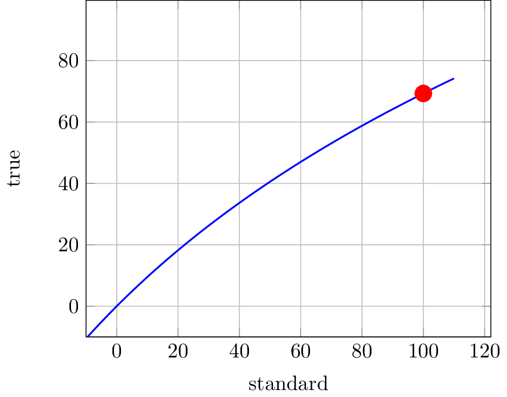
Until, say, 20%, there is not much difference, but for higher increases, the difference is significant.

Observe for instance that a true increase of \(70\%\) is associated to a standard increase of \(100\%\); this is exactly the “rule of 70” which is explained later.

Our new definition leads to a fundamental result:

Some examples of usage:

• An increase of \(1000\%\) followed by an increase of \(1000\%\) is exactly an increase of \(2000\%\)
• An increase of \(50\%\) followed by a decrease of \(50\%\) is exactly an increase of \(0\%\) (so, a multiplication by one)

Rates

This new way of computing increases is even more important for time dependent increases. In that case, one talks about rates, which is an increase per unit of time. (This is actually called the “continuously compounded rate”)

So a rate of \(x\%\) per year (or “per annum”) means a multiplication by \(\exp(tx/100)\) where \(t\) is in years.

• An increase of \(5.2\%\) per year means a multiplication by \(1.0533\) every year (this is the current interest rate of the US central bank)
• An increase of \(70\%\) per year means a multiplication by \(2\) every year.

Who needs compounding?

So, suppose you know the rate, but you leave your money in a savings account for three years instead of one. What is you gain after three years? Well, it is another growth coefficient, which can also be described in percents.

Let us use the standard rate \(r\) first. After one year, you have \(1+r\) and after three years, you have \((1+r)^3\). That is a new growth factor, equal to some other standard rate \(r'\), that is \(r' = (1+r)^3-1\). For instance, if \(r = 10%\), then, after three years, you can compute that \(r' = 33\%\), so slightly more than \(3 r\).

Let's use the true rate \(R\) instead. After one year, by definition, the growth is \(\ee^{R}\), so after three years, the growth is just \(\ee^{3R}\), which means that the true rate is after three years, exactly three times that of one year. Dead simple! In the last example, the true rate was \(R = 9.53\%\), after three years, it is simply \(R' = 3R\), so \(R' =3 \times 9.53\%\). That's it!

What this means is: the unit of a true rate is the same as units of frequencies (inverse of time). Once you know the rate in one unit, a rescaling gives the rate in any other units. If a frequency is \(f = 1/\text{s}\) (the heart beat frequency), then for a minute, which is \(60s\), the same frequency is simply \(f = 60/\text{min}\)

This works exactly the same for (true) rates:

• A monthly rate of \(x\%\) is exactly a yearly rate of \(12x\%\).
• A daily rate of \(x\%\) is exactly a yearly rate of \(365x\%\)

This explains the title of this post: compounding only exists because of ignorance of exponentials.

The rule of 70%

One way to get a feeling of a given growth rate is how long before it doubles? If the rate is negative, this is the same idea, and is called the half life of whatever is decaying. Mathematically, the solution is obtained by simply solving \(G^T = 2\), which gives \(T = \log(2)/\log(G)\).

So using the true rate \(R\), expressed in percents, and using the approximation \(\log(2) \approx 70%\), we get \[ T \approx 70\%/R \] This formula is exact even for very large rates (except for the approximation \(\log(2) \approx 70\%\))! For example, a true rate \(R = 70\%\) implies \(T = 1\) which means that the growing quantity doubles every year.

The formula is still true for standard rates, if they are small, since we have the relation \(R = \log(1+r) \approx r\) when \(r\) is small.

Some Applications

Yield and Forward Rates

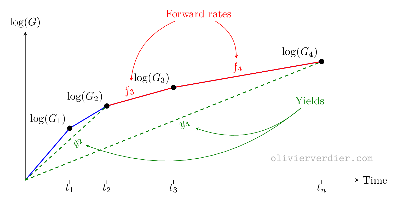
Here is the basic setting. Through a market of government bonds (“Zero coupon bonds”), either directly existing or constructed artificially, the growth of money can be broken down as follows.

Suppose we have “maturities” \(t_0,t_1,t_2,\ldots,t_N\) (we take the convention that \(t_0 = 0\)) and corresponding growth factors \(g_1\) from \(t_0\) to \(t_1\), and generally \(g_k\) between \(t_{k-1}\) to \(t_k\).

So, the growth factor between \(t_0\) and \(t_k\) is \(G_k\): \[ G_k = g_1\cdots g_k \]

What is measured is the price of zero-coupon bonds (for a nominal of one), which, for a maturity \(t_k\) is exactly \(1/G_k\).

Let us define the time intervals \[Δt_k := t_k - t_{k-1}\]

These growth coefficients give rise to “forward rates”: \[ f_k := \log(g_k)/Δt_{k}\]

What is called the yield \(y_k\) for maturity \(t_k\) is, with our conventions, \[y_k = \log(G_k)/(t_k - t_0)\]

A picture best summarises all these definitions:

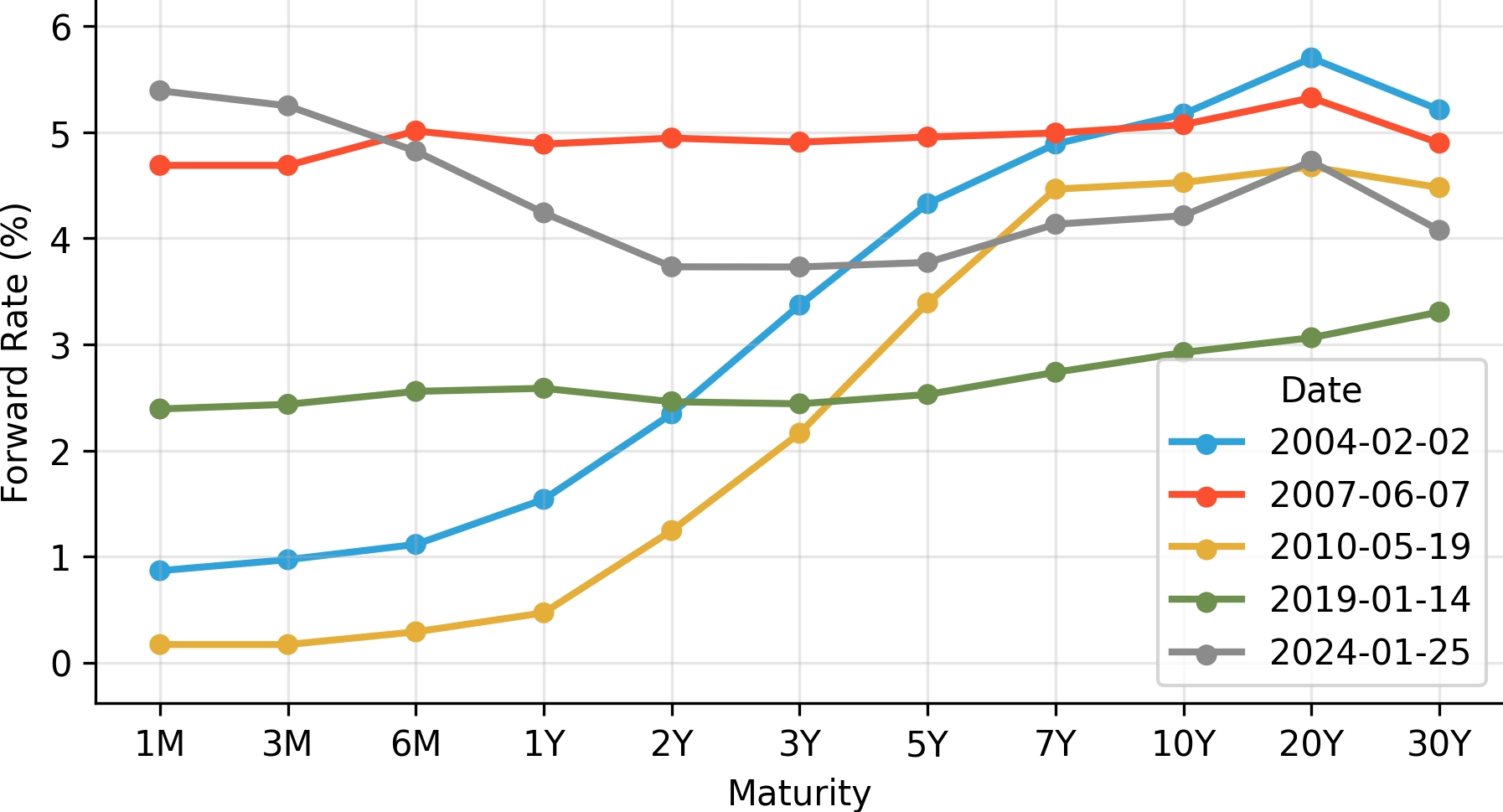
Here is a couple of forward rates of US treasury bonds computed at some interesting dates:

Forward Rate Agreement

We make the assumption that at times \(t_k\) and \(t_{k+1}\), there is a possibility to borrow money, at a rate \(L_k\). To simplify the notations, we write \[ α := Δt_{k+1} := t_{k+1}-t_k\]

A forward rate agreement with strike \(K\) is the agreement (made before time \(t_k\)) to pay \(\exp(α K) -1\) and receive \(\exp(αL_k) - 1\) at time \(t_{k+1}\). The payout at time \(t_{k+1}\) is thus \[ \exp(αL_k) - \exp(αK) \]

The growth at time \(t_k\) is denoted by \(G_k\). The price of the corresponding bond is \(1/G_k\).

The forward libor rate is the strike \(K\) at which the value of the forward rate agreement is zero.

Consider a portfolio consisting of

• one unit of a zero coupon bond maturing at \(t_k\)
• \(-\exp(αK)\) units of zero coupon bonds maturing at \(t_{k+1}\).

At time \(t_k\), one can put the one unit coming from the zero coupon bond at \(t_k\) in a deposit, which gives us at time \(t_{k+1}\) the value \(\exp(αL_{k})\). So at time \(t_{k+1}\), the value of the portfolio is equal to \(\exp(αL_{k}) - \exp(αK)\), which is precisely the payoff of the forward rate agreement.

The present value \(V_K\) of the portfolio is thus the present value \(V_K\) of the forward rate agreement, and it is equal to \[ V_K = 1/G_k - \exp(αK)/G_{k+1} \]

The value of the strike \(K\) which gives \(V_K = 0\) is given by \[ K = \log(G_{k+1}/G_k)/α \]

In other words, that value is exactly the forward rate between \(t_k\) and \(t_{k+1}\).

Bond Durations

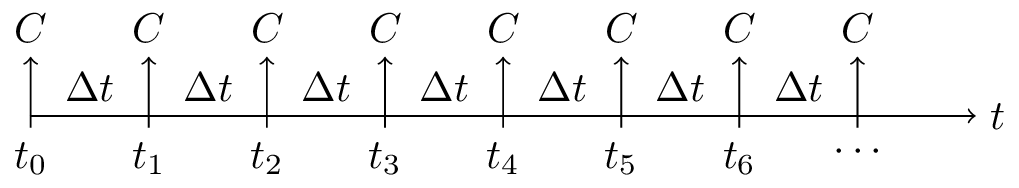
Another case where true rates are useful are bonds. A bond is a financial instrument that brings the bearer fixed cash flows across a given period. The intermediate cash flows are called coupons. A zero-coupon bond a special bond which pays only once. The last payment occurs at a time called the maturity of the bond.

What has any of this to do with exponentials?

Zero-coupon Bonds: one cash flow, finite maturity

Let us look at the zero-coupon case first. Suppose it brings a cash-flow of \(C_T\) at maturity (time) \(T\).

Such a bond has a price \(P\). This, in turn, determines a growth factor from \(P\) to \(C_T\), in a time period of \(T\). There is a true rate \(Y\) defined by \(Y = \log(C_T/P)/T\). This the standard associated rate is called the yield, let us call this the true yield \(Y\).

A fundamental assumption of finance is that, if this is a risk free bond, for instance a government bond, this yield gives the price of money at a given maturity \(T\). In other words, any future cash flow \(C\) at that time \(T\) has, as of today, a discounted value, or present value of \(\exp(-YT) C\).

By definition, the price obeys the rule \(P(Y) = C_T \exp(-YT)\). We focus on the yield-price relationship: it is decreasing (i.e., \(P'(Y) ≤ 0\)) and convex (i.e., \(P''(Y) ≥ 0\)).

What happens if we compute the derivative of the function \(P(Y)\)? We get \(P'(Y) = -T P(Y)\), so it is natural to call the quantity \[ D(Y) := -P'(Y)/P(Y)\] the duration of the bond. Here, the duration \(D(Y)\) is independent of \(Y\) and equal to the maturity \(T\): \(D(Y) = T\).

General Bonds: more cash flows, finite maturity

Let us see what happens with more complicated cash flows.

Suppose we get a cash flow of \(C_{t_k}\) at time points \(t_k\).

Suppose we know the yield for some maturity \(T\), and here, let us make the following simplifying assumption:

(Yields are typically not constant, as was explained above, but sometimes, when the forward rates are constant, so are the yields)

The value of a bond is then, as explained above, the discounted value of the cash flows at the given times \(t_k\).

We thus get \(P(Y) = \sum_k \exp(-Yt_k) C_{t_k} \). Define the weights \[p_k(Y) := \frac{\exp(-Yt_k) C_{t_k}}{P} \] which have the property that \(\sum_k p_k(Y) = 1\) and \(p_k(Y) ≥ 0\), assuming each cash flow \(C_{t_k}\) to be nonnegative. Define the duration with the same formula as above, i.e., \(D(Y) = -P'(Y)/P(Y)\) and obtain \(D(Y) = \frac{\sum_k t_k \exp(-Yt_k) C_{t_k}}{\sum_k \exp(-Yt_k) C_{t_k}} \), that is \[ D(Y) = \sum_k p_k(Y) t_k \] This formula shows that the duration is a weighted average of the cash-flow times \(t_k\). This implies for instance that the duration is always lower than the maturity.

Annuity: regular cash flows, infinite maturity

In fact, for an annuity, that is, a bond with infinite maturity, one can compute a finite duration as follows. Suppose for simplicity that \(t_k = k Δt\), which means that the cash flow comes at regular time intervals \(Δt\), and that \(C_{t_k} = C\), which means that the cash flow is constant.

First, the price \(P(Y)\) is \begin{align} x &= 0 \\ y &= 0 \end{align} \begin{align} P(Y) &= C \sum_{k=0}^{∞} \exp(-YΔt k) \\ &= \frac{C}{1-\exp(-Y Δt)} \end{align} Now, since the duration was \(D(Y) = -P'(Y)/P(Y)\), or \(D(Y) = (\log(1/P(Y)))'\), which means \(D(Y) = (\log(1-\exp(-YΔt)))'\), We obtain \[ D(Y) = \frac{Δt}{\exp(Δt Y) - 1} \] which is clearly a finite time!

In fact, one can define the function \[ Φ(x) := \frac{\exp(x) - 1}{x} \] which is prolonged at \(x = 0\) by continuity, so \(Φ(0) = 1\). The annuity duration becomes \[ D(Y) = \frac{1}{Y Φ(Δt Y)} \] This shows that the only way for an annuity duration to become infinite is for the true yield \(Y\) to approach zero.