The idea of this post is to show that the classical relations of thermodynamics are simple consequences of elementary probability theory, and in particular of exponential families.

The mathematical setting is thus the same as for exponential families.

There are several isolated systems, each of which equipped with a space of microstates $X$, with a support measure $δx$.

We will say that a state is now a probability distribution $π$ over $X$.

General Setup

We start with systems with no macroscopic variables (such as volume).

We also assume that there is an energy function \[ E \colon X \to \RR \]

We will call internal energy of the system the mean energy of that sytem at the given state $π$:

\[ \mathsf{U}(π) := \langle π, E \rangle \]

Entropy Law

Recall that the entropy of a state $π$ is defined by

\[ \mathsf{S}(π) := \langle π , -\log(π) \rangle \]

Let us start with the most fundamental principle.

Entropy Law

The state $π$ of a system at equilibrium maximises entropy at a given value $U$ of the internal energy. The equilibrium state $π'$ is thus \[ π' := \operatorname{argmax}_{\mathsf{U}(π) = U} \mathsf{S}(π) \]

The consequence is that at equilibrium, there is a number $θ$ such that the state $π$ is a density of the form

\[ π_{θ}(x) := \exp\Big(E(x) θ - A(θ)\Big) \]

We interpret $θ$ as the temperature of the system. The temperature $θ$ and the value of the internal energy $U$ are closely connected as we shall see shortly.

The (log)partition function $A(θ)$, which serves as a normalisation factor in the probability distribution $π_{θ}$, is defined by

\[ A(θ) := \log \Big( \int_{X} \exp(E(x) θ) δ x\Big) \]

Note that we know from general facts about exponential families that

$A$ is convex

Besides, again from these general facts, we know that

\[ \frac{∂A}{∂θ} = U \]

(Note that we put a partial derivative purely in preparation of what comes later, namely dependency on another variable; for the moment, this is just a standard derivative of a real valued function on a a subset of $\RR$).

What is that subset of $\RR$? Well, the domain of definition $Θ$ consists of the temperatures for which this function exists, which is precisely

\[ Θ := \Big\{θ \subset \RR \mid \int_{X} \exp(E(x)) δ x < ∞\Big\} \]

So we see that the temperature $θ$ and the corresponding internal energy value $U$ are related by the relation above. The take home message about this is that convexity of the normalisation function $A$ means that if the temperature $θ$ increases, then the internal energy $U$ increases as well.

Phase Transitions

In this model, the partition function $A$ is strictly convex. However, in reality, an increase of internal energy does not lead to an increase of temperature (but the temperature cannot decrease, due to convexity). When that happens, this is called a first order phase transition.

Chemical Potentials

In most of this presentation, we do not really assume that the temperature is scalar. Indeed, the general setting is that the “energy function” represents in fact both the energy but also the concentrations of the various chemical components. This gives a function of the form \[ F(x) = (E(x), N_1(x),\ldots,N_n(x)) \] for $n$ chemical components. The “temperature” associated to any of those concentrations $N_i$ is called a chemical potential. For simplicity, we will present thermodynamics without these potentials.

Thermal Contact

Suppose now that, two of these systems are put in contact. This creates a new system with space \[ X = X_1 \cup X_2 \] The new energy function is \[ E(x_1,x_2) := E_1(x_1) + E_2(x_2) \] The state of the new system is \[ π(x_1,x_2) := π_1(x_1) π_2(x_2) \] which is automatically a probability density.

The internal energy of the new system is thus \[ U = \langle π, E \rangle = \langle π_1, E_1 \rangle + \langle π_2, E_2 \rangle \]

This new system is not at equilibrium (in general). Indeed, for now the state is just \[ π(x_1, x_2) = \exp(θ_1 E_1(x) + θ_2 E_2(x) - A_1(θ_1) - A_2(θ_2)) \] In fact, it is not in equilibrium unless the temperatures $θ_1$ and $θ_2$ were equal. According to the entropy law, the system will settle to a new state $π'$ a temperature $θ$ such that \[ π'(x_1, x_2) = \exp(θ E(x) - A(θ)) \]

Direct Derivation of Temperature equilibrium

Here is an alternative way to see that the temperatures must be equal. This is not needed, though, as we already know the form of the density with highest entropy. Since \[ U = \int_{X_1 \times X_2} (E_1(x_1) + E_2(x_2)) π_1(x_1) π_2(x_2) δx_1 δx_2 = U_1 + U_2 \] and \[ \dd S = \dd S_1 + \dd S_2 = \frac{∂S_1}{∂U_1} \dd U_1 + \frac{∂S_2}{∂U_2} \dd U_2 = \dd U_2 (θ_1 - θ_2) \] we conclude that for maximum entropy to be achieved, both temperatures have to be equal.

A calculation shows that \[ A(θ) = A_1(θ) + A_2(θ) \] The constraint is that, the equilibrium state $π'$ is such that \[ \mathsf{U}(π') = U_1 + U_2 \] From the identities relating the internal energy and the normalisation functions, we get \[ A_1'(θ) + A_2'(θ) = A'_1(θ_1) + A'_2(θ_2) \] We reformulate this as \[ {\frac{A'_1(θ) - A'_1(θ_1)}{θ - θ_1}} (θ - θ_1) = \frac{A'_2(θ_2) - A'_2(θ)}{θ_2 - θ} (θ_2 - θ) \]

Now, we know, by convexity, that both $A'_1$ and $A'_2$ are non-decreasing functions. So if we define \[ α_1 := \frac{A'_1(θ) - A'_1(θ_1)}{θ - θ_1} \] and \[ α_2 := \frac{A'_2(θ_2) - A'_2(θ)}{θ_2 - θ} \] we have that $α_1 ≥ 0$ and $α_2 ≥ 0$, as well as \[ θ = \frac{α_1}{α_1 + α_2} θ_1 + \frac{α_2}{α_1 + α_2} θ_2 \]

We conclude that, supposing for instance that $θ_1 ≤ θ_2$, then we have

\[ θ_1 ≤ θ ≤ θ_2 \]

Macroscopic Variables

We now assume that the energy function may depend on an external macroscopic variable that we denote by $V$, as it is essentially the volume in practice: $E \colon X \times Y \to \RR$. We note the energy function $E_V \colon X \to \RR$ for a fixed macroscopic value, denoted by $V$.

The (mean) energy $\mathsf{U}$ of a given state $π$ is then

\[ \mathsf{U}(π,V) := \langle π, E_V \rangle = \int E_V(x) π(x) δx \]

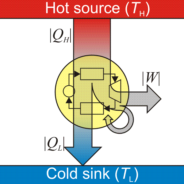
Heat and Work

During a smooth change, we obtain by differentiation the

First Law of thermodynamics

\[ \dd \mathsf{U} = \underbrace{\frac{∂\mathsf{U}}{∂V} \dd V}_{δW} + \underbrace{\frac{∂\mathsf{U}}{∂π} \dd π}_{δQ} \]

Using the product rule, we obtain that the work $δW$ is defined by

\[ δW := \int \frac{∂E_V}{∂V} (x) π(x) δx \dd V \]

and the heat $δQ$ is defined by

\[ δQ := \int E_V(x) \dd π(x) δx \]

This is useful because we want to decrease the energy of the system in exchange for work. In other words, $δW ≤ 0$ means that the energy of the system is decreased, so this energy is transmitted to the outside world.

Differential Forms?

If we regard the complete manifold of states, spanned by distributions $π$ on $X$ and a macroscopic variable $V$, then heat $δQ$ and $δW$ are differential forms on that manifold.

Pressure

We can also define the pressure, for a general state $π$ and macroscopic variable $V$ as

\[ \mathsf{p}(π, V) := - \Big\langle π, \frac{∂E_V}{∂V}(x) \Big\rangle \]

Equilibrium

As we saw before, at equilibrium, the state $π$ must take the form $π_{θ,V}$ with

\[ π_{θ,V}(x) := \exp\Big(E_V(x) θ - A_V(θ)\Big) \]

As before, the partition function $A_V(θ)$ is defined by \[ A_V(θ) := \log \Big( \int \exp(E_V(x) θ) δ x\Big) \] Again, the domain of definition $Θ_V$ consists of the temperatures for which this function exists, which is precisely \[ Θ_V := \Big\{θ \mid \int \exp(θ E_V(x)) δ x < ∞\Big\} \]

So now,

The variables $(θ,V)$ parameterize the manifold of equilibria.

We will denote

\[ \mathcal{F}(θ,V) := A_V(θ) \]

and call $\mathcal{F}(θ,V)$ the free energy for the temperature $θ$.

Recall that the entropy of a distribution $π$ is defined by \[ \mathsf{S}(π) := \langle π, -\log(π) \rangle = \int -\log(π(x)) π(x) δx \]

Let us denote the equilibrium entropy by

\[\mathcal{S}(θ, V) := \mathsf{S}(π_{θ,V})\]

We also define the equilibrium internal energy as

\[ \mathcal{U}(θ,V) := \mathsf{U}(π_{θ,V}, V) \]

From general properties of exponential families, we immediately get: \[ \mathcal{U}(θ,V) = \frac{∂{A_{V}}}{∂θ}(θ,V) \] and by convexity of $A_V$: \[ \frac{∂^2 \mathcal{F}}{∂θ^2} ≥ 0 \] We also have the convexity equality relating the free energy $\mathcal{F}$, the entropy $\mathcal{S}$, the internal energy $\mathcal{U}$ and the temperature $θ$.

\[ \mathcal{F}(θ,V) - \mathcal{S}(θ,V) = θ \mathcal{U}(θ,V) \]

Heat and Entropy

From the definition of the entropy $\mathsf{S}$, and using that $π$ is a probability distribution, we get \[ \dd \mathsf{S} = \int -\log(π(x)) \dd π(x) δx \]

Supposing the reversibility assumption, meaning that $π$ always stays at maximum entropy, it must then be an exponential distribution $π_{θ,V}$, so \[ \dd \mathsf{S} = \int (A(θ) - E_V(x)θ) \dd π δx = - \int E_V(x) θ \dd π δ x = - θ δQ \]

Finally, during a reversible change, we have $\mathsf{S}(π_{θ,V}) = \mathcal{S}(θ,V)$, so we get the fundamental relation between entropy, heat and temperature,

\[ \dd \mathcal{S} = - θ δQ \]

Is energy free?

Here we see an indication of the terminology “free energy” for $\mathcal{F}$: at constant temperature $θ$, the free energy $\mathcal{F}$ is a proxy for work. Indeed, by differentiation, and using the identities above, we have, for a reversible change: \[ \dd \mathcal{F} = θ δW + \mathcal{U} \dd θ \] so, for an isothermic transformation, $\dd \mathcal{F} = θ δW$.

Differential Geometry Black Magic

The manifold of equilibria $\Man$ is the subset spanned by the variables $(θ,V)$, that is, the set

\[ \Man := \{(θ, V) \in \RR \times Y \mid θ \in Θ_V \} \]

We call macrostates the parameters $θ,V$ of the manifold $\Man$.

So this is just a restriction of the more general internal energy function $\mathsf{U}$ which was defined on all states, not only the ones at equilibrium.

We can always define a new function from an old one. Let us first define the pressure. It could be defined for any state $π$ but we will restrict the definition on the equilibrium states. So, if $π$ is an equilibrium state, them during a reversible change, $δW = -p \dd V$. This defines the function $p$ on the manifold of macrostates.

Let us define the pressure at equilibrium by \[ p(θ,V) := \mathsf{p}(π_{θ,V}, V) \] For a reversible change, we thus obtain

\[ θ \dd \mathcal{U} = -θ p \dd V - \dd \mathcal{S} \]

We can now define the enthalpy on the manifold of macrostates as \[ \mathcal{H}(θ,V) := \mathcal{U}(θ,V) + p(θ,V) V \]

This is just another function. The magic comes from differentiation:

\[ θ \dd \mathcal{H} = θ V \dd p - \dd \mathcal{S} \]

It is important to remember that $p$ and $\mathcal{S}$ are functions, not variables. There is no guarantees that these can be used as variables to parameterize the manifold of equilibria. Also, this definition of the enthalpy has nothing much to do with the Legendre transform.

Positive Temperature

Until now, the value of the temperature $θ$ depends on the energy functions $E_v$. We make the following assumption

Assumption

Assume that for each value of $V$, $E_V$ is bounded from below and that \[ \int_X δx > ∞ \]

These assumptions have a simple consequence, the temperature is positive, in the sense that our temperature $θ$ is negative:

\[ θ < 0 \]

or, equivalently, \[ Θ_V \subset (-∞, 0) \]

Indeed, we know that for any fixed $V$, the domain $Θ_V$ is convex. Moreover, the assumption above makes sure that $0 \not\in Θ_V$.

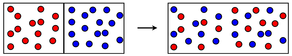
Irreversible Change

Let us imagine a scenario of irreversible change.

Assume that a part of the states suddently becomes accessible, with no other changes.

The microstate $p$ will then stop being in equilibrium, but will move to the highest entropy given this new configuration. The main observation is now that moving the system back to its original configuration will require lowering the entropy.

If we assume that \[ E_V(x) ≥ 0 \] it means that \[ θ ≤ 0 \] and a decrease of entropy $\dd S ≤ 0$ means a decrease of energy due to heat. This energy is constant, it means in the end an increase of energy due to work to compensate from that.

We get the result

Theorem

On a cycle with irreversible change, the total work put in the system must be positive (in other words: no work can be obtained from an irreversible cycle)

Summary

There is a space of states, which is a set of probability distributions $π$ over a set of microstates $X$.

Some functions are defined over all possible states:

internal energy $\mathsf{U}$
entropy $\mathsf{S}$
pressure $\mathsf{p}$

Some differential forms are defined over that manifold of states:

the work differential $δW$
the heat differential $δQ$

There is a statistical manifold of equilibria which is a submanifold consisting of the distributions $π_{θ,V}$.

Some functions are naturally defined on the manifold of equilibria:

obviously, the temperature $θ$
free energy $\mathcal{F}(θ, V)$
enthalpy $\mathcal{H}(θ,V)$

As the name suggest, if a state is not at equilibrium, it will spontaneously go to the corresponding equilibrium state with the same mean energy. This corresponds to maximising the entropy.

References

Two sources of inspiration were:

Making Sense of the Legendre Transform by Zia, Redish and McKay.
Topics in Statistical Mechanics by Brian Cowan, and a corresponding course page with slides and other material.

Another interesting reference is Concepts in Thermal Physics.

Edit 2021-11: This is pretty much a complete rewrite, as the previous version was rather incomplete.